 Visual Paradigm Desktop |
  Visual Paradigm Online


System Performance Prediction is a critical milestone in the lifecycle of complex engineering projects. Without accurate models, teams rely on physical prototypes, which are costly and time-consuming to modify. SysML (Systems Modeling Language) offers a standardized approach to represent system behavior and structure. By leveraging behavioral modeling techniques, engineers can simulate scenarios before hardware is built. This guide explores how to apply SysML behavioral diagrams to predict performance outcomes effectively.
Model-Based Systems Engineering (MBSE) shifts the focus from documents to models. In this context, behavioral modeling defines how a system acts over time. It captures interactions, state changes, and data flows. For performance prediction, behavior is not just about functionality; it is about timing, resource consumption, and throughput.
Behavioral modeling in SysML serves several key purposes:
When predicting performance, the goal is to quantify variables such as latency, energy usage, or throughput. SysML diagrams provide the structural framework for these calculations. The language is designed to be tool-agnostic, ensuring that models remain valid regardless of the platform used for simulation.
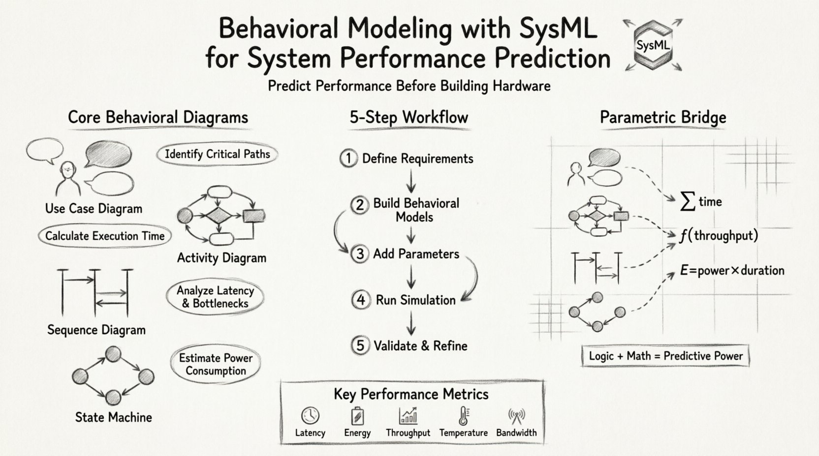
SysML includes several diagram types specifically designed to capture system behavior. Each diagram serves a unique role in the performance prediction workflow. Selecting the right diagram depends on the specific aspect of performance being analyzed.
Use Case Diagrams define the functional scope of the system. They map actors to the functions they interact with. While primarily used for functional requirements, they set the stage for performance analysis by identifying high-level interactions.
For performance prediction, Use Case Diagrams help identify critical paths. If a specific actor interacts frequently with a high-load function, that path requires detailed timing analysis.
Activity Diagrams describe the flow of control and data within the system. They are the most direct tool for modeling processes and workflows. In performance engineering, these diagrams map the sequence of operations.
Key elements include:
When simulating performance, Activity Diagrams allow for the calculation of total execution time. By assigning time values to individual activities, the total duration of a process becomes a calculable metric. This is essential for real-time systems where latency is a critical constraint.
Sequence Diagrams focus on the interaction between components over time. They display messages exchanged between objects along a timeline. This diagram type is vital for understanding communication overhead.
Performance considerations for Sequence Diagrams include:
By analyzing the vertical axis (time), engineers can identify bottlenecks in inter-component communication. This is particularly useful for distributed systems where network latency impacts overall performance.
State Machine Diagrams model the lifecycle of a system or component. They define distinct states and the transitions that occur between them. Performance prediction here focuses on state duration and transition frequency.
Key aspects include:
In performance analysis, State Machine Diagrams help calculate power consumption. Different states often have different power profiles. By modeling the probability of being in a specific state, engineers can estimate average energy usage over time.
Behavioral diagrams describe what the system does. To predict performance, we must quantify how well it does it. This is where Parametric Diagrams become essential. They link the behavioral model to mathematical constraints and equations.
Parametric Diagrams are the bridge between logical behavior and physical performance. They allow engineers to define constraints using algebraic expressions. These constraints are then used by simulation engines to solve for unknown variables.
Common parameters analyzed include:
By associating parameters with specific elements in behavioral diagrams, the model becomes a simulation-ready asset. For example, an activity in an Activity Diagram can be linked to a time parameter in a Parametric Diagram. When the simulation runs, the engine calculates the actual duration based on the defined equations.
Creating a predictive model requires a structured approach. Adhering to a consistent workflow ensures accuracy and maintainability. The following steps outline the process of integrating behavioral modeling with performance prediction.
Before modeling begins, performance goals must be established. These are often expressed as constraints. Examples include:
These requirements are recorded in the Requirements Diagram. They serve as the baseline for validating the simulation results later.
Create the logical representation of the system. Start with Use Case Diagrams to define scope. Then, develop Activity Diagrams for high-level processes. Use Sequence Diagrams for detailed interactions. Ensure that all relevant states are captured in State Machine Diagrams.
At this stage, focus on correctness. The logic must be sound before performance metrics are added. A flawed logic model will produce flawed performance data.
Link the behavioral elements to performance parameters. Use Parametric Diagrams to define the mathematical relationships. For instance, link the execution time of an activity to a variable representing processor speed and task complexity.
Run the model using a simulation engine. The engine processes the constraints and behavioral logic to generate data. This data is then compared against the performance requirements defined in Step 1.
Key activities during this phase include:
Compare simulation results with real-world data if available. If the model predicts 100ms latency but the prototype shows 150ms, the model needs refinement. Update the parameters or logic to align with physical reality.
Choosing the right diagram is crucial for efficient modeling. Not all diagrams are suitable for every performance aspect. The table below outlines the strengths and limitations of each diagram type in the context of performance prediction.
| Diagram Type | Primary Focus | Performance Metric | Best Used For |
|---|---|---|---|
| Use Case | Functional Scope | Interaction Frequency | Identifying high-load use cases |
| Activity | Process Flow | Total Execution Time | Calculating cycle times and throughput |
| Sequence | Component Interaction | Latency & Message Overhead | Network and inter-process communication analysis |
| State Machine | Lifecycle & States | Power & State Duration | Estimating energy consumption and idle times |
| Parametric | Mathematical Constraints | Quantitative Metrics | Linking logic to physical performance values |
Building behavioral models for performance prediction involves specific challenges. Recognizing these early helps prevent rework and model inaccuracies.
Attempting to model every detail can make the simulation intractable. High complexity increases computation time and obscures critical insights.
Mitigation: Use abstraction. Model at the level of detail required for the specific performance question. Simplify non-critical paths.
Simulation requires accurate input data. If parameters like processor speed or network latency are unknown, the results will be speculative.
Mitigation: Use ranges and sensitivity analysis. Define best-case, worst-case, and average-case scenarios to account for uncertainty.
SysML behavior models are often static representations of dynamic systems. Capturing real-time changes can be difficult.
Mitigation: Combine behavioral diagrams with external simulation tools. Use SysML for logic and structure, and specialized tools for high-fidelity physics or network simulation.
To ensure the longevity and utility of behavioral models, follow these best practices.
Requirements are the foundation of performance prediction. Without clear requirements, there is no benchmark for success. SysML supports this through the Requirements Diagram.
Effective requirement modeling includes:
When a requirement specifies a performance limit, it should be linked to the relevant parameter in the Parametric Diagram. This creates an automated verification path. If the simulation violates the constraint, the model flags the requirement as unmet.
Performance prediction is rarely isolated. It often intersects with software, hardware, and physical engineering. SysML facilitates this integration through standardized interfaces.
Software performance depends on the underlying hardware and system architecture. SysML models can define the software allocation to hardware components. This allows for the simulation of software load on specific processors.
Hardware constraints such as power supply and thermal dissipation directly affect performance. Parametric Diagrams can link system behavior to hardware specifications. This ensures that the design remains feasible within physical limits.
For systems involving motion or fluid dynamics, physical constraints must be modeled. While SysML handles logic well, it often integrates with domain-specific simulation tools for complex physics. The interface between the behavioral model and the physics engine is critical.
The field of Systems Modeling Language continues to evolve. As systems become more complex, the demand for accurate performance prediction grows.
Behavioral Modeling with SysML provides a robust framework for System Performance Prediction. By combining logical diagrams with mathematical constraints, engineers can validate designs before physical realization. The process requires careful planning, accurate data, and a clear understanding of the system’s operational context.
Key points to remember:
Adopting this approach reduces risk and cost while improving system reliability. It enables teams to make informed decisions based on data rather than intuition. As systems grow in complexity, the ability to predict performance through modeling becomes an essential capability for engineering success.
Yes, SysML models can be simulated if they include the necessary behavioral logic and parametric constraints. However, the complexity of the simulation depends on the specific tools used and the depth of the model.
Functional modeling defines what the system does. Performance modeling defines how well it does it. SysML allows both to be modeled within the same framework, ensuring alignment between function and capability.
Use ranges and probabilistic methods. Define minimum, maximum, and expected values for parameters. Run simulations with different combinations to understand the impact of uncertainty on the final result.
By following these guidelines, teams can build effective behavioral models that drive better engineering outcomes. The investment in modeling pays off through reduced prototyping cycles and higher confidence in system performance.